Contents
qgraph
qgraph
BIG 5 DATASET
# Load big5 dataset:
data(big5)
data(big5groups)
# Correlations:
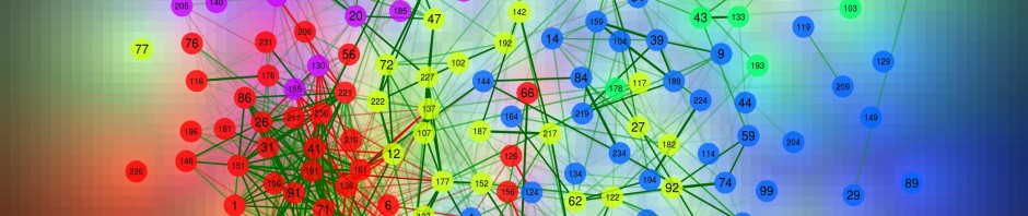
Q <- qgraph(cor(big5), minimum = 0.25, cut = 0.4, vsize = 1.5, groups = big5groups,
legend = TRUE, borders = FALSE)
title("Big 5 correlations", line = 2.5)

# Same graph with spring layout:
Q <- qgraph(Q, layout = "spring")
title("Big 5 correlations", line = 2.5)

# Same graph with Venn diagram overlay:
qgraph(Q, overlay = TRUE)
title("Big 5 correlations", line = 2.5)

# Same graph with different color scheme:
qgraph(Q, posCol = "blue", negCol = "purple")
title("Big 5 correlations", line = 2.5)

# Significance graph (circular):
qgraph(Q, graph = "sig", layout = "circular")
title("Big 5 correlations (p-values)", line = 2.5)

# Significance graph:
qgraph(Q, graph = "sig")
title("Big 5 correlations (p-values)", line = 2.5)

# Significance graph (distinguishing positive and negative statistics):
qgraph(Q, graph = "sig2")
title("Big 5 correlations (p-values)", line = 2.5)

# Grayscale graphs:
qgraph(Q, gray = TRUE, layout = "circular")
title("Big 5 correlations", line = 2.5)

qgraph(Q, graph = "sig", gray = TRUE)
title("Big 5 correlations (p-values)", line = 2.5)

# Correlations graph with scores of random subject:
qgraph(cor(big5), minimum = 0.25, cut = 0.4, vsize = 1.5, groups = big5groups,
legend = TRUE, borders = FALSE, scores = as.integer(big5[sample(1:500, 1),
]), scores.range = c(1, 5))
title("Test scores of random subject", line = 2.5)

layout(1)
# EFA:
big5efa <- factanal(big5, factors = 5, rotation = "promax", scores = "regression")
qgraph(big5efa, groups = big5groups, layout = "circle", rotation = "promax",
minimum = 0.2, cut = 0.4, vsize = c(1.5, 15), borders = FALSE, vTrans = 200)
title("Big 5 EFA", line = 2.5)

# PCA:
library("psych")
big5pca <- principal(cor(big5), 5, rotate = "promax")
qgraph(big5pca, groups = big5groups, layout = "circle", rotation = "promax",
minimum = 0.2, cut = 0.4, vsize = c(1.5, 15), borders = FALSE, vTrans = 200)
title("Big 5 PCA", line = 2.5)

UNWEIGHTED DIRECTED GRAPHS
set.seed(1)
adj = matrix(sample(0:1, 10^2, TRUE, prob = c(0.8, 0.2)), nrow = 10, ncol = 10)
qgraph(adj)
title("Unweighted and directed graphs", line = 2.5)

# Save plot to nonsquare pdf file:
qgraph(adj, filetype = "pdf", height = 5, width = 10)
EXAMPLES FOR EDGES UNDER DIFFERENT ARGUMENTS
# Create edgelist:
dat.3 <- matrix(c(1:15 * 2 - 1, 1:15 * 2), , 2)
dat.3 <- cbind(dat.3, round(seq(-0.7, 0.7, length = 15), 1))
# Create grid layout:
L.3 <- matrix(1:30, nrow = 2)
# Different esize:
qgraph(dat.3, layout = L.3, directed = FALSE, edge.labels = TRUE, esize = 14)

# Different esize, strongest edges omitted (note how 0.4 edge is now just
# as wide as 0.7 edge in previous graph):
qgraph(dat.3[-c(1:3, 13:15), ], layout = L.3, nNodes = 30, directed = FALSE,
edge.labels = TRUE, esize = 14)

# Different esize, with maximum:
qgraph(dat.3, layout = L.3, directed = FALSE, edge.labels = TRUE, esize = 14,
maximum = 1)
title("maximum=1", line = 2.5)

qgraph(dat.3[-c(1:3, 13:15), ], layout = L.3, nNodes = 30, directed = FALSE,
edge.labels = TRUE, esize = 14, maximum = 1)
title("maximum=1", line = 2.5)

# Different minimum
qgraph(dat.3, layout = L.3, directed = FALSE, edge.labels = TRUE, esize = 14,
minimum = 0.1)
title("minimum=0.1", line = 2.5)

# With cutoff score:
qgraph(dat.3, layout = L.3, directed = FALSE, edge.labels = TRUE, esize = 14,
cut = 0.4)
title("cut=0.4", line = 2.5)

# With details:
qgraph(dat.3, layout = L.3, directed = FALSE, edge.labels = TRUE, esize = 14,
minimum = 0.1, maximum = 1, cut = 0.4, details = TRUE)
title("details=TRUE", line = 2.5)

Additional topics
# Trivial example of manually specifying edge color and widths:
E <- as.matrix(data.frame(from = rep(1:3, each = 3), to = rep(1:3, 3), width = 1:9))
qgraph(E, mode = "direct", edge.color = rainbow(9))

pcalg support
# Example from pcalg vignette:
library("pcalg")
data(gmI)
suffStat <- list(C = cor(gmI$x), n = nrow(gmI$x))
pc.fit <- pc(suffStat, indepTest = gaussCItest, p = ncol(gmI$x), alpha = 0.01)
qgraph(pc.fit)
qgraph.cfa
# Simulate dataset:
set.seed(2)
eta <- matrix(rnorm(200 * 5), ncol = 5)
lam <- matrix(rnorm(50 * 5, 0, 0.15), 50, 5)
lam[apply(diag(5) == 1, 1, rep, each = 10)] <- rnorm(50, 0.7, 0.3)
th <- matrix(rnorm(200 * 50), ncol = 50)
Y <- eta %*% t(lam) + th
# Create groupslist
gr <- list(1:10, 11:20, 21:30, 31:40, 41:50)
# Using 'lavaan' package:
res <- qgraph.cfa(cov(Y), N = 200, groups = gr, pkg = "lavaan", vsize.man = 2,
vsize.lat = 10)

qgraph.lavaan(res, filename = "lavaan", legend = FALSE, groups = gr, edge.label.cex = 0.6)
## [1] "Output stored in /home/sacha/Documents/phd/R/lavaan.pdf"
# Using 'sem' package:
res <- qgraph.cfa(cov(Y), N = 200, groups = gr, pkg = "sem", vsize.man = 2,
vsize.lat = 10, fun = qgraph.loadings)

qgraph.semModel(res, edge.label.cex = 0.6)

qgraph(res, edge.label.cex = 0.6)

qgraph.sem(res, filename = "sem", legend = FALSE, groups = gr, edge.label.cex = 0.6)
## [1] "Output stored in /home/sacha/Documents/phd/R/sem.pdf"
Big 5 dataset
data(big5)
data(big5groups)
fit <- qgraph.cfa(cov(big5), nrow(big5), big5groups, pkg = "lavaan", opts = list(se = "none"),
vsize.man = 1, vsize.lat = 6, edge.label.cex = 0.5)

print(fit)
## lavaan (0.5-11) converged normally after 128 iterations
##
## Number of observations 500
##
## Estimator ML
## Minimum Function Test Statistic 60838.192
## Degrees of freedom 28430
## P-value (Chi-square) 0.000
qgraph.layout.fruchtermanreingold
# This example makes a multipage PDF that contains images Of a building
# network using soft constraints.
# Each step one node is added with one edge. The max.delta decreases the
# longer nodes are present in the network.
pdf("Soft Constraints.pdf", width = 10, height = 5)
adj = adjO = matrix(0, nrow = 3, ncol = 3)
adj[upper.tri(adj)] = 1
Q = qgraph(adj, vsize = 3, height = 5, width = 10, layout = "spring", esize = 1,
filetype = "", directed = T)
cons = Q$layout
for (i in 1:20) {
x = nrow(adj)
adjN = matrix(0, nrow = x + 1, ncol = x + 1)
adjN[1:x, 1:x] = adj
consN = matrix(NA, nrow = x + 1, ncol = 2)
consN[1:x, ] = cons[1:x, ]
layout.par = list(init = rbind(cons, c(0, 0)), max.delta = 10/(x + 1):1,
area = 10^2, repulse.rad = 10^3)
y = sample(c(x, sample(1:(x), 1)), 1)
adjN[y, x + 1] = 1
Q = qgraph(adjN, Q, layout = "spring", layout.par = layout.par)
cons = Q$layout
adj = adjN
}
dev.off()
## pdf
## 2
qgraph_loadings
# Load big5 dataset:
data(big5)
data(big5groups)
big5efa <- factanal(big5, factors = 5, rotation = "promax", scores = "regression")
big5loadings <- loadings(big5efa)
qgraph.loadings(big5loadings, groups = big5groups, rotation = "promax", minimum = 0.2,
cut = 0.4, vsize = c(1.5, 15), borders = FALSE, vTrans = 200)

# Tree layout:
qgraph.loadings(big5loadings, groups = big5groups, rotation = "promax", minimum = 0.2,
cut = 0.4, vsize = c(1.5, 15), borders = FALSE, vTrans = 200, layout = "tree",
width = 20, filetype = "R")
qgraph_svg
VISUALIZE CORRELATION MATRIX
eta = matrix(rnorm(200 * 5), ncol = 5)
lam = matrix(0, nrow = 100, ncol = 5)
for (i in 1:5) lam[(20 * i - 19):(20 * i), i] = rnorm(20, 0.7, 0.3)
eps = matrix(rnorm(200 * 100), ncol = 100)
Y = eta %*% t(lam) + eps
tooltips = paste("item", 1:100)
groups = list(1:20, 21:40, 41:60, 61:80, 81:100)
names(groups) = paste("Factor", LETTERS[1:5])
# Run qgraph:
qgraph_pca
data(big5)
data(big5groups)
qgraph.pca(cor(big5), 5, groups = big5groups, rotation = "promax", minimum = 0.2,
cut = 0.4, vsize = c(1, 7), borders = FALSE, vTrans = 200)

# Tree layout:
qgraph.pca(cor(big5), 5, groups = big5groups, rotation = "promax", minimum = 0.2,
cut = 0.4, vsize = c(1.5, 15), borders = FALSE, layout = "tree", width = 20,
filetype = "R")
qgraph_efa
data(big5)
data(big5groups)
qgraph.efa(big5, 5, groups = big5groups, rotation = "promax", minimum = 0.2,
cut = 0.4, vsize = c(1, 7), borders = FALSE, vTrans = 200)

# Tree layout:
qgraph.efa(big5, 5, groups = big5groups, rotation = "promax", minimum = 0.2,
cut = 0.4, vsize = c(1, 7), borders = FALSE, layout = "tree", width = 20,
filetype = "R")
qgraph.panel
data(big5)
data(big5groups)
qgraph.panel(cor(big5), groups = big5groups, minimum = 0.2, borders = FALSE,
vsize = 1, cut = 0.3)

centrality
set.seed(1)
adj <- matrix(sample(0:1, 10^2, TRUE, prob = c(0.8, 0.2)), nrow = 10, ncol = 10)
Q <- qgraph(adj)

centrality(Q)
## $OutDegree
## [1] 3 2 0 2 1 2 2 1 2 2
##
## $InDegree
## [1] 3 1 2 1 1 1 2 4 0 2
##
## $Closeness
## [1] 0.00 0.00 0.00 0.00 0.00 0.00 0.00 0.00 0.04 0.00
##
## $Betweenness
## [1] 28 13 0 12 12 12 10 13 0 14
##
## $ShortestPathLengths
## [,1] [,2] [,3] [,4] [,5] [,6] [,7] [,8] [,9] [,10]
## [1,] 0 3 1 2 1 4 1 2 Inf 3
## [2,] 2 0 3 4 3 1 3 1 Inf 5
## [3,] Inf Inf 0 Inf Inf Inf Inf Inf Inf Inf
## [4,] 1 3 2 0 2 4 2 2 Inf 1
## [5,] 2 4 3 1 0 5 3 3 Inf 2
## [6,] 1 2 2 3 2 0 2 1 Inf 4
## [7,] 1 2 2 3 2 3 0 1 Inf 4
## [8,] 3 1 4 5 4 2 4 0 Inf 6
## [9,] 3 3 1 5 4 4 2 2 0 1
## [10,] 2 2 3 4 3 3 1 1 Inf 0
##
## $ShortestPaths
## [,1] [,2] [,3] [,4] [,5] [,6] [,7] [,8] [,9]
## [1,] List,0 List,1 List,1 List,1 List,1 List,1 List,1 List,1 List,0
## [2,] List,1 List,0 List,1 List,1 List,1 List,1 List,1 List,1 List,0
## [3,] List,0 List,0 List,0 List,0 List,0 List,0 List,0 List,0 List,0
## [4,] List,1 List,1 List,1 List,0 List,1 List,1 List,2 List,1 List,0
## [5,] List,1 List,1 List,1 List,1 List,0 List,1 List,2 List,1 List,0
## [6,] List,1 List,1 List,1 List,1 List,1 List,0 List,1 List,1 List,0
## [7,] List,1 List,1 List,1 List,1 List,1 List,1 List,0 List,1 List,0
## [8,] List,1 List,1 List,1 List,1 List,1 List,1 List,1 List,0 List,0
## [9,] List,1 List,1 List,1 List,1 List,1 List,1 List,1 List,1 List,0
## [10,] List,1 List,1 List,1 List,1 List,1 List,1 List,1 List,1 List,0
## [,10]
## [1,] List,1
## [2,] List,1
## [3,] List,0
## [4,] List,1
## [5,] List,1
## [6,] List,1
## [7,] List,1
## [8,] List,1
## [9,] List,1
## [10,] List,0